Session 3: Data Frames
Topics
- Data frames
- Input from and output to files
- Exploring data frames
- Clean up data frames
- Adding and modifying columns in a data frame
- Summarizing data with bar plots
Getting data into R
Let’s revisit the chunk of code that we started out with at the beginning of the last lesson
library(tidyverse)
library(readxl)

pcoa <- read_tsv(file="raw_data/baxter.braycurtis.pcoa.axes")
metadata <- read_excel(path="raw_data/baxter.metadata.xlsx")
metadata_pcoa <- inner_join(metadata, pcoa, by=c('sample'='group'))

ggplot(metadata_pcoa, aes(x=axis1, y=axis2, color=dx)) +
	geom_point(shape=19, size=2) +
	scale_color_manual(name=NULL,
		values=c("blue", "red", "black"),
		breaks=c("normal", "adenoma", "cancer"),
		labels=c("Normal", "Adenoma", "Cancer")) +
	coord_fixed() +
	labs(title="PCoA of Bray-Curtis Distances Between Stool Samples",
		x="PCo Axis 1",
		y="PCo Axis 2") +
	theme_classic()

ggsave("ordination.pdf")
After loading the tidyverse and readxl packages, there are two lines where we read in data:
pcoa <- read_tsv(file="raw_data/baxter.braycurtis.pcoa.axes")
metadata <- read_excel(path="raw_data/baxter.metadata.xlsx")
These two lines read in our ordination data and the data about the samples represented in the ordination (i.e. metadata). The first line uses the function, read_tsv to read in a tab separated values-formatted file. As the name suggests, this function will read in a file where the columns in the file are separated by tab characters. This function comes from the readr package that was loaded as part of the tidyverse package. This package also has functions for reading in comma sseparated values (CSVs) files (read_csv), general delimited files (read_delim), fixed width files (read_fwf), and file where columns are separated by whitespace (read_table). As the name suggests, the second line of code relies on the read_excel function from the readxl package to read a table in from a Microsoft Excel-formatted spreadsheet. Within the tidyverse, there are the haven package, which can be used to read in SAS, SPSS, and Stata-formatted files. There are a number of other reading packages that aren’t specifically part of the tidyverse, but that do allow you to read in data from websites, databases, and other sources**.
Each of these functions has a decent number of options that default to values that make sense. Be careful - there are other similarly named functions (e.g. read.tsv) that are actually built into R and have different defaults that don’t make sense. What are the defaults? What options can we change? Remember from the last lesson that we can use the ? to get the documentation for any function
?read_tsv
read_delim                package:readr                R Documentation

Read a delimited file (including csv & tsv) into a tibble

Description:

     ‘read_csv()’ and ‘read_tsv()’ are special cases of the general
     ‘read_delim()’. They're useful for reading the most common types
     of flat file data, comma separated values and tab separated
     values, respectively. ‘read_csv2()’ uses ‘;’ for separators,
     instead of ‘,’. This is common in European countries which use ‘,’
     as the decimal separator.

Usage:

     read_delim(file, delim, quote = "\"", escape_backslash = FALSE,
       escape_double = TRUE, col_names = TRUE, col_types = NULL,
       locale = default_locale(), na = c("", "NA"), quoted_na = TRUE,
       comment = "", trim_ws = FALSE, skip = 0, n_max = Inf,
       guess_max = min(1000, n_max), progress = show_progress())

     read_csv(file, col_names = TRUE, col_types = NULL,
       locale = default_locale(), na = c("", "NA"), quoted_na = TRUE,
       quote = "\"", comment = "", trim_ws = TRUE, skip = 0, n_max = Inf,
       guess_max = min(1000, n_max), progress = show_progress())

     read_csv2(file, col_names = TRUE, col_types = NULL,
       locale = default_locale(), na = c("", "NA"), quoted_na = TRUE,
       quote = "\"", comment = "", trim_ws = TRUE, skip = 0, n_max = Inf,
       guess_max = min(1000, n_max), progress = show_progress())

     read_tsv(file, col_names = TRUE, col_types = NULL,
       locale = default_locale(), na = c("", "NA"), quoted_na = TRUE,
       quote = "\"", comment = "", trim_ws = TRUE, skip = 0, n_max = Inf,
       guess_max = min(1000, n_max), progress = show_progress())

Arguments:

    file: Either a path to a file, a connection, or literal data
          (either a single string or a raw vector).

          Files ending in ‘.gz’, ‘.bz2’, ‘.xz’, or ‘.zip’ will be
          automatically uncompressed. Files starting with ‘http://’,
          ‘https://’, ‘ftp://’, or ‘ftps://’ will be automatically
          downloaded. Remote gz files can also be automatically
          downloaded and decompressed.

          Literal data is most useful for examples and tests. It must
          contain at least one new line to be recognised as data
          (instead of a path).

   delim: Single character used to separate fields within a record.

   quote: Single character used to quote strings.

escape_backslash: Does the file use backslashes to escape special
          characters? This is more general than ‘escape_double’ as
          backslashes can be used to escape the delimiter character,
          the quote character, or to add special characters like ‘\n’.

escape_double: Does the file escape quotes by doubling them? i.e. If
          this option is ‘TRUE’, the value ‘""""’ represents a single
          quote, ‘\"’.

col_names: Either ‘TRUE’, ‘FALSE’ or a character vector of column
          names.

          If ‘TRUE’, the first row of the input will be used as the
          column names, and will not be included in the data frame. If
          ‘FALSE’, column names will be generated automatically: X1,
          X2, X3 etc.

          If ‘col_names’ is a character vector, the values will be used
          as the names of the columns, and the first row of the input
          will be read into the first row of the output data frame.

          Missing (‘NA’) column names will generate a warning, and be
          filled in with dummy names ‘X1’, ‘X2’ etc. Duplicate column
          names will generate a warning and be made unique with a
          numeric prefix.
<snipped>
This is the documentation for four readr commands: read_delim, read_csv, read_csv2, and read_tsv. They differ by the delimeter that they use to separate columns. For the most part, the defaults are what you will want. The only exception may be the col_names option, which defaults to TRUE indicating that your file has column headings. If our file didn’t have headings, we’d use the following syntax:
# Don't run this!
pcoa <- read_tsv(file="raw_data/baxter.braycurtis.pcoa.axes", col_names=FALSE)
These reading functions are pretty smart and can generally figure out the type of data that is in each column.
Activity 1
Pretend that the data we want is actually on the second page of the data/baxter.metadata.xlsx workbook. Can you rewrite the read_excel command to read that page?
Activity 2
Open one of the spreadsheets where you keep the metadata for your project
- What do you see in your spreadsheet that might cause problems?
- How would you want to organize your metadata to make it easier to use with R?
- Look at the formatting of your data. Are all of the dates consistently formatted? Do you use a consistent capitalization style? Do you use non-text information (e.g. color) to represent values?
The output of the read functions that are part of the tidyverse are a special type of data frame called a tibble. To back up a step, what is a data frame? A data frame can be thought of as a table where each row represents a different entity and each column represents a different aspect of that entity. For example, the metadata variable stores the value of a data frame where each row represents a different person and each column represents various attributes of those people whether its their subject identification number, weight, height, location, diagnosis, smoking status, etc. Each row has the same number of columns. If a piece of data is missing, then R will denote the value for that entity with the NA value. Got it? Moving on, a tibble is a special type of data frame that is a stripped down version of the data.frame structure that is core to R. Keeping with the . for _ theme, data_frame can be used as an alias for tibble.
There are some special aspects of a tibble to be aware of. Perhaps most important is that there are no names on the rows. Not allowing names on the rows is a safety measure to protect you from some weird quirks in R. Another difference is when you enter the name of the data frame at the prompt, instead of having the entire data frame vomited at your screen, you get an abbreviated output:
metadata
## # A tibble: 490 x 17
##    sample fit_result Site  Dx_Bin dx    Hx_Prev Hx_of_Polyps   Age Gender Smoke
##     <dbl>      <dbl> <chr> <chr>  <chr>   <dbl>        <dbl> <dbl> <chr>  <dbl>
##  1 2.00e6          0 U Mi… High … norm…       0            1    64 m         NA
##  2 2.01e6          0 U Mi… High … norm…       0            1    61 m          0
##  3 2.01e6         26 U Mi… High … norm…       0            1    47 f          0
##  4 2.01e6         10 Toro… Adeno… aden…       0            1    81 f          1
##  5 2.01e6          0 U Mi… Normal norm…       0            0    44 f          0
##  6 2.02e6          0 Dana… High … norm…       0            1    51 f          1
##  7 2.02e6          7 Dana… Cancer canc…       1            1    78 m          1
##  8 2.02e6         19 U Mi… Normal norm…       0            0    59 m          0
##  9 2.02e6          0 Dana… High … norm…       1            1    63 f          1
## 10 2.03e6       1509 U Mi… Cance… canc…       1            1    67 m          1
## # … with 480 more rows, and 7 more variables: Diabetic <dbl>, Hx_Fam_CRC <dbl>,
## #   Height <dbl>, Weight <dbl>, NSAID <dbl>, Diabetes_Med <dbl>, stage <dbl>
The output gives me the first ten columns and the first ten rows of the data frame. You’ll notice that at the top of the output, it tells us that there are 490 rows and 17 columns. The column headings for the 7 columns that weren’t outputted are listed at the bottom of the output. It also indicates, that 480 rows were not included in the output. In addition, the output tells us what type of variable each column contains. For example, the fit_result column contains dbl or double precision numbers and the dx column contains chr or character values. You’ll also notice that zero values have a lighter color and that the NA for the first value in the Smoke column is red. These are all meant to improve the visualization of the data.
Activity 3
Compare the output from typing metadata at the prompt to the output of typing as.data.frame(metadata) at the prompt.
Exploring our metadata
Let’s dig into the metadata to think about how we’d like to use it to improve our scatter plot or perhaps visualize the variation in our cohort. Whenever we read in a data frame there are a few things to do get a handle on your data. First, as we’ve already done, entering the name of the data frame at the prompt will tell us a lot of information. We might also want to get access to those individual chunks of data
nrow(metadata)
## [1] 490
ncol(metadata)
## [1] 17
dim(metadata)
## [1] 490 17
These three commands tell us the number of rows (nrow), columns (ncol), and both together (dim) in our metadata data frame. Let’s find out the names of our columns
colnames(metadata)
##  [1] "sample"       "fit_result"   "Site"         "Dx_Bin"       "dx"
##  [6] "Hx_Prev"      "Hx_of_Polyps" "Age"          "Gender"       "Smoke"
## [11] "Diabetic"     "Hx_Fam_CRC"   "Height"       "Weight"       "NSAID"
## [16] "Diabetes_Med" "stage"
Are these column names informative? What type of information do you think each column might contain? If our data frame had names on the rows, we could get their value using the rownames command in a similar way. We can get a sense of the data frame using the head command, which returns the first 6 values of a variable or tail, which returns the last 6 values.
head(metadata)
## # A tibble: 6 x 17
##   sample fit_result Site  Dx_Bin dx    Hx_Prev Hx_of_Polyps   Age Gender Smoke
##    <dbl>      <dbl> <chr> <chr>  <chr>   <dbl>        <dbl> <dbl> <chr>  <dbl>
## 1 2.00e6          0 U Mi… High … norm…       0            1    64 m         NA
## 2 2.01e6          0 U Mi… High … norm…       0            1    61 m          0
## 3 2.01e6         26 U Mi… High … norm…       0            1    47 f          0
## 4 2.01e6         10 Toro… Adeno… aden…       0            1    81 f          1
## 5 2.01e6          0 U Mi… Normal norm…       0            0    44 f          0
## 6 2.02e6          0 Dana… High … norm…       0            1    51 f          1
## # … with 7 more variables: Diabetic <dbl>, Hx_Fam_CRC <dbl>, Height <dbl>,
## #   Weight <dbl>, NSAID <dbl>, Diabetes_Med <dbl>, stage <dbl>
tail(metadata)
## # A tibble: 6 x 17
##   sample fit_result Site  Dx_Bin dx    Hx_Prev Hx_of_Polyps   Age Gender Smoke
##    <dbl>      <dbl> <chr> <chr>  <chr>   <dbl>        <dbl> <dbl> <chr>  <dbl>
## 1 3.53e6          0 Dana… Normal norm…       0            0    51 f          0
## 2 3.53e6          0 Dana… Normal norm…       1            0    53 f          0
## 3 3.54e6          0 U Mi… Adv A… aden…       0            1    75 m          1
## 4 3.54e6          0 U Mi… Normal norm…       0            0    56 f          0
## 5 3.55e6          0 Dana… Adeno… aden…       1            1    77 m          1
## 6 3.56e6          0 U Mi… Normal norm…       0            0    51 f          0
## # … with 7 more variables: Diabetic <dbl>, Hx_Fam_CRC <dbl>, Height <dbl>,
## #   Weight <dbl>, NSAID <dbl>, Diabetes_Med <dbl>, stage <dbl>
We can also use the glimpse command to get an idea about the structure of a variable.
glimpse(metadata)
## Rows: 490
## Columns: 17
## $ sample       <dbl> 2003650, 2005650, 2007660, 2009650, 2013660, 2015650, 20…
## $ fit_result   <dbl> 0, 0, 26, 10, 0, 0, 7, 19, 0, 1509, 0, 0, 0, 0, 0, 72, 0…
## $ Site         <chr> "U Michigan", "U Michigan", "U Michigan", "Toronto", "U …
## $ Dx_Bin       <chr> "High Risk Normal", "High Risk Normal", "High Risk Norma…
## $ dx           <chr> "normal", "normal", "normal", "adenoma", "normal", "norm…
## $ Hx_Prev      <dbl> 0, 0, 0, 0, 0, 0, 1, 0, 1, 1, 0, 0, 0, 1, 0, 0, 0, 0, 0,…
## $ Hx_of_Polyps <dbl> 1, 1, 1, 1, 0, 1, 1, 0, 1, 1, 0, 1, 1, 0, 0, 0, 1, 1, 1,…
## $ Age          <dbl> 64, 61, 47, 81, 44, 51, 78, 59, 63, 67, 65, 55, 72, 77, …
## $ Gender       <chr> "m", "m", "f", "f", "f", "f", "m", "m", "f", "m", "f", "…
## $ Smoke        <dbl> NA, 0, 0, 1, 0, 1, 1, 0, 1, 1, 0, 1, 1, 0, 0, 0, 1, 1, 1…
## $ Diabetic     <dbl> 0, 0, 0, 0, 0, 0, 1, 0, 0, 0, 0, 0, 0, 0, 1, 0, 0, 0, 0,…
## $ Hx_Fam_CRC   <dbl> 1, 0, 1, 0, 0, 0, 0, 0, 0, 0, 0, 1, 0, 1, 0, 0, 0, 1, 1,…
## $ Height       <dbl> 182, 167, 170, 168, 170, 160, 172, 177, 154, 167, 167, 1…
## $ Weight       <dbl> 120, 78, 63, 65, 72, 67, 78, 65, 54, 58, 60, 90, 57, 68,…
## $ NSAID        <dbl> 0, 0, 0, 1, 1, 0, 0, 0, 0, 0, 0, 1, 0, 0, 0, 0, 0, 1, 1,…
## $ Diabetes_Med <dbl> 0, 0, 0, 0, 0, 0, 1, 0, 0, 0, 0, 0, 0, 0, 1, 0, 0, 0, 0,…
## $ stage        <dbl> 0, 0, 0, 0, 0, 0, 3, 0, 0, 4, 0, 0, 0, 0, 0, 3, 0, 0, 0,…
You’ll commonly encounter numerical (dbl, int, or num), categorical (fctr), boolean (lgl), and text (chr) data. The str command will tell you the type of data you have in your variable.
Another function that is great for characterizing a data frame (or any type of variable) is summary.
summary(metadata)
##      sample          fit_result         Site              Dx_Bin
##  Min.   :2003650   Min.   :   0.0   Length:490         Length:490
##  1st Qu.:2326158   1st Qu.:   0.0   Class :character   Class :character
##  Median :2776662   Median :   0.0   Mode  :character   Mode  :character
##  Mean   :2757494   Mean   : 236.3
##  3rd Qu.:3155185   3rd Qu.: 102.5
##  Max.   :3561650   Max.   :2964.0
##
##       dx               Hx_Prev        Hx_of_Polyps         Age
##  Length:490         Min.   :0.0000   Min.   :0.0000   Min.   :29.00
##  Class :character   1st Qu.:0.0000   1st Qu.:0.0000   1st Qu.:52.00
##  Mode  :character   Median :0.0000   Median :1.0000   Median :60.00
##                     Mean   :0.2834   Mean   :0.6687   Mean   :60.28
##                     3rd Qu.:1.0000   3rd Qu.:1.0000   3rd Qu.:69.00
##                     Max.   :1.0000   Max.   :1.0000   Max.   :89.00
##                     NA's   :3        NA's   :1
##     Gender              Smoke           Diabetic        Hx_Fam_CRC
##  Length:490         Min.   :0.0000   Min.   :0.0000   Min.   :0.0000
##  Class :character   1st Qu.:0.0000   1st Qu.:0.0000   1st Qu.:0.0000
##  Mode  :character   Median :0.0000   Median :0.0000   Median :0.0000
##                     Mean   :0.4587   Mean   :0.1166   Mean   :0.1694
##                     3rd Qu.:1.0000   3rd Qu.:0.0000   3rd Qu.:0.0000
##                     Max.   :1.0000   Max.   :1.0000   Max.   :1.0000
##                     NA's   :6        NA's   :1
##      Height          Weight           NSAID         Diabetes_Med
##  Min.   :  0.0   Min.   :  0.00   Min.   :0.0000   Min.   :0.00000
##  1st Qu.:162.0   1st Qu.: 67.00   1st Qu.:0.0000   1st Qu.:0.00000
##  Median :170.0   Median : 78.00   Median :0.0000   Median :0.00000
##  Mean   :169.8   Mean   : 79.08   Mean   :0.2459   Mean   :0.08163
##  3rd Qu.:177.0   3rd Qu.: 90.00   3rd Qu.:0.0000   3rd Qu.:0.00000
##  Max.   :203.0   Max.   :193.00   Max.   :1.0000   Max.   :1.00000
##  NA's   :1       NA's   :1        NA's   :2
##      stage
##  Min.   :0.0000
##  1st Qu.:0.0000
##  Median :0.0000
##  Mean   :0.5245
##  3rd Qu.:0.0000
##  Max.   :4.0000
##
Activity 4
What do you notice about the output of running glimpse(metadata)? What types of data are there? Thinking about the list of data types outlined above, are there columns that are improperly formatted? Do the column names match the type of data in the column? Looking at the output of summary(metadata), what do you notice about how the different data types were summarized?
Cleaning our metadata
After a quick look at the metadata we can see that there are a few things that aren’t quite right that we might want to fix. Some of the columns are the wrong type and some of the values in the data frame don’t make sense. For example, the sample column is a double and it should be a character. Let’s start by fixing the column types. There are multiple ways to do this, but it is probably easiest, in the long run, to use the col_types argument in read_excel and read_tsv. Unfortunately, they have slightly different syntax. For read_excel the col_type options are “skip”, “guess”, “logical”, “numeric”, “date”, “text” or “list”. We’ll normally only use “logical”, “numeric”, “text”, and “date”. It is important to list the column types in order. Although we provide the column names for the col_types value, read_excel doesn’t actually look at these values. Including them helps me to organize the column types when there are more than a handful of columns.
metadata <- read_excel(path="raw_data/baxter.metadata.xlsx",
		col_types=c(sample = "text", fit_result = "numeric", Site = "text", Dx_Bin = "text",
				dx = "text", Hx_Prev = "logical", Hx_of_Polyps = "logical", Age = "numeric",
				Gender = "text", Smoke = "logical", Diabetic = "logical", Hx_Fam_CRC = "logical",
				Height = "numeric", Weight = "numeric", NSAID = "logical", Diabetes_Med = "logical",
				stage = "text")
	)
metadata
## # A tibble: 490 x 17
##    sample fit_result Site  Dx_Bin dx    Hx_Prev Hx_of_Polyps   Age Gender Smoke
##    <chr>       <dbl> <chr> <chr>  <chr> <lgl>   <lgl>        <dbl> <chr>  <lgl>
##  1 20036…          0 U Mi… High … norm… FALSE   TRUE            64 m      NA
##  2 20056…          0 U Mi… High … norm… FALSE   TRUE            61 m      FALSE
##  3 20076…         26 U Mi… High … norm… FALSE   TRUE            47 f      FALSE
##  4 20096…         10 Toro… Adeno… aden… FALSE   TRUE            81 f      TRUE
##  5 20136…          0 U Mi… Normal norm… FALSE   FALSE           44 f      FALSE
##  6 20156…          0 Dana… High … norm… FALSE   TRUE            51 f      TRUE
##  7 20176…          7 Dana… Cancer canc… TRUE    TRUE            78 m      TRUE
##  8 20196…         19 U Mi… Normal norm… FALSE   FALSE           59 m      FALSE
##  9 20236…          0 Dana… High … norm… TRUE    TRUE            63 f      TRUE
## 10 20256…       1509 U Mi… Cance… canc… TRUE    TRUE            67 m      TRUE
## # … with 480 more rows, and 7 more variables: Diabetic <lgl>, Hx_Fam_CRC <lgl>,
## #   Height <dbl>, Weight <dbl>, NSAID <lgl>, Diabetes_Med <lgl>, stage <chr>
In contrast, if we used read_tsv the syntax would look like this (note that this won’t run since you don’t have data/baxter.metadata.tsv)
metadata <- read_tsv(file="raw_data/baxter.metadata.tsv",
		col_types=cols(sample = col_character(), fit_result = col_double(), Site = col_character(),
				Dx_Bin = col_character(), dx = col_character(), Hx_Prev = col_logical(),
				Hx_of_Polyps = col_logical(), Age = col_integer(), Gender = col_character(),
				Smoke = col_logical(), Diabetic = col_logical(), Hx_Fam_CRC = col_logical(),
				Height = col_double(), Weight = col_double(), NSAID = col_logical(),
				Diabetes_Med = col_logical(), stage = col_character())
	)
This is a bit tedious, but once you’ve done it you won’t need to do it again. Also we can see exactly how we have recast the various columns to the correct format. I would strongly discourage editing the original metadata file to correct these problems. For example, you could do a find-all-replace-all to change 0 values in the “Diabetic” column to FALSE and the 1 values to TRUE. In the long run, this is likely to create more problems than it solves. Your raw data should stay raw. This is an advantage of using a function like read_excel - my collaborator can send me their workbook and I can use it as they gave it to me without mucking it up. Using the data munging procedures we’re in the midst of, I can programmatically change the file without changing the version I have on my hard drive. This allows me to always know the provenience of my data.
Now that we have the types of variables correct, let’s re-run the summary function to see how things look
summary(metadata)
Take a moment to look at the columns represented in your data frame and the information presented below the column names. Do all of the values seem reasonable? Need a hint? Check out the information below “Height” and “Weight”. Think someone could weight 0 kg or be 0 cm tall? I think those should instead be NA. We need to learn a few concepts before we can convert the 0 values to NA values. First, we need to know how to modify individual columns or create new columns. We can do this with the mutate function:
mutate(metadata, age_in_months = Age * 12)
mutate(metadata, Height = Height/100)
The mutate function takes the metadata data frame and adds a new column that is the age of the person in months. Similarly, the second command edits the Height column to change it from centimeters to meters. If we do the following, what do you notice?
metadata
## # A tibble: 490 x 17
##    sample fit_result Site  Dx_Bin dx    Hx_Prev Hx_of_Polyps   Age Gender Smoke
##    <chr>       <dbl> <chr> <chr>  <chr> <lgl>   <lgl>        <dbl> <chr>  <lgl>
##  1 20036…          0 U Mi… High … norm… FALSE   TRUE            64 m      NA
##  2 20056…          0 U Mi… High … norm… FALSE   TRUE            61 m      FALSE
##  3 20076…         26 U Mi… High … norm… FALSE   TRUE            47 f      FALSE
##  4 20096…         10 Toro… Adeno… aden… FALSE   TRUE            81 f      TRUE
##  5 20136…          0 U Mi… Normal norm… FALSE   FALSE           44 f      FALSE
##  6 20156…          0 Dana… High … norm… FALSE   TRUE            51 f      TRUE
##  7 20176…          7 Dana… Cancer canc… TRUE    TRUE            78 m      TRUE
##  8 20196…         19 U Mi… Normal norm… FALSE   FALSE           59 m      FALSE
##  9 20236…          0 Dana… High … norm… TRUE    TRUE            63 f      TRUE
## 10 20256…       1509 U Mi… Cance… canc… TRUE    TRUE            67 m      TRUE
## # … with 480 more rows, and 7 more variables: Diabetic <lgl>, Hx_Fam_CRC <lgl>,
## #   Height <dbl>, Weight <dbl>, NSAID <lgl>, Diabetes_Med <lgl>, stage <chr>
Next, do you see that we don’t have age_in_months as a column and the values in our Height column don’t appear to be in meters? Why is that? Right! We didn’t assign the modified data frames back to metadata. We won’t do that with these two changes, but this is an important point to remember. The data frame will only change if we assign the new data frame to the name of the old data frame. Finally, the dplyr package, which is one of the core package within the tidyverse, has a useful function called na_if. If it finds a value we specify in the vector, it will convert it to an NA.
metadata <- mutate(metadata, Height = na_if(Height, 0))
metadata <- mutate(metadata, Weight = na_if(Weight, 0))
Running summary(metadata) again, we see that the ranges for the “Height” and “Weight” columns are more reasonable now. We’d like to look at the values for our columns that contain character values, but they’re obfuscated. One way to check this out is with the count command
count(metadata, Site)
## # A tibble: 5 x 2
##   Site              n
##   <chr>         <int>
## 1 Dana Farber     120
## 2 MD Anderson      95
## 3 Toronto         168
## 4 U Michigan      106
## 5 U of Michigan     1
count(metadata, Dx_Bin)
## # A tibble: 6 x 2
##   Dx_Bin               n
##   <chr>            <int>
## 1 Adenoma             89
## 2 Adv Adenoma        109
## 3 Cancer             119
## 4 Cancer.              1
## 5 High Risk Normal    50
## 6 Normal             122
count(metadata, dx)
## # A tibble: 3 x 2
##   dx          n
##   <chr>   <int>
## 1 adenoma   198
## 2 cancer    120
## 3 normal    172
count(metadata, Gender)
## # A tibble: 2 x 2
##   Gender     n
##   <chr>  <int>
## 1 f        243
## 2 m        247
count(metadata, stage)
## # A tibble: 5 x 2
##   stage     n
##   <chr> <int>
## 1 0       370
## 2 1        39
## 3 2        35
## 4 3        36
## 5 4        10
Notice anything weird here? Yup. In the “Site” column, it looks like our collaborator used “U of Michigan” for one subject, but “U Michigan” for all of the others. We need to fix this. We can use the dplyr function recode to make this easy…
metadata <- mutate(metadata, Site = recode(.x=Site, "U of Michigan"="U Michigan"))
count(metadata, Site)
## # A tibble: 4 x 2
##   Site            n
##   <chr>       <int>
## 1 Dana Farber   120
## 2 MD Anderson    95
## 3 Toronto       168
## 4 U Michigan    107
Activity 5
You should notice that in the “Dx_Bin” column there is a subject with the value “Cancer.” rather than “Cancer”. Using recode, can you fix this value?
Activity 6
It might be obvious to us what is contained in the “Gender” column - “f” and “m” are the only two values. What if we wanted to make the values a little more meaningful and have them read as “female” and “male”? Write a recode function(s) to convert the single character to the longer name. Confirm that you get the correct result
Cleaning up column names
If we look back at our column names in the metadata data frame, you’ll notice that some names are in title case (e.g. “Hx_Prev”) and others are in all lower case (e.g. “fit_result”). Also, some of the column names may not make sense to you if you aren’t a clinican (e.g. “Hx_Prev”). You may have also noticed that our “Gender” column has data regarding the subject’s sex, not gender. Let’s see how we can fix these issues to make using the data frame easier.
As I mentioned above, there are two problems with the name “Hx_Prev” - the capitalization is inconsistent with the other columns and it may not be immediately clear what “Hx_Prev” means. We have many options for how to name things. “Hx_Prev” could be written as “HxPrev”, “hxPrev”, “hx_prev”, “hx.prev”, “previous_history”, etc. It can get confusing to remember which column headings are capitalized and which are not. The general preference in the R world is to use lowercase lettering and to separate words in a name with an underscore (i.e. _). This is called “snake case”. Having a consistent capitalization strategy may seem a bit pedantic, but it makes it easier to keep your names straight when you don’t have to worry about capitalization. The preference would be to change names like “Site” and “Hx_Prev” to “site” and “hx_prev”. We can convert the column names to lower case using the rename_all function in the dplyr package with the tolower function. Conversely, if you wanted everything in all caps, you could use the toupper function
metadata <- rename_all(.tbl=metadata, .funs=tolower)
metadata
## # A tibble: 490 x 17
##    sample fit_result site  dx_bin dx    hx_prev hx_of_polyps   age gender smoke
##    <chr>       <dbl> <chr> <chr>  <chr> <lgl>   <lgl>        <dbl> <chr>  <lgl>
##  1 20036…          0 U Mi… High … norm… FALSE   TRUE            64 male   NA
##  2 20056…          0 U Mi… High … norm… FALSE   TRUE            61 male   FALSE
##  3 20076…         26 U Mi… High … norm… FALSE   TRUE            47 female FALSE
##  4 20096…         10 Toro… Adeno… aden… FALSE   TRUE            81 female TRUE
##  5 20136…          0 U Mi… Normal norm… FALSE   FALSE           44 female FALSE
##  6 20156…          0 Dana… High … norm… FALSE   TRUE            51 female TRUE
##  7 20176…          7 Dana… Cancer canc… TRUE    TRUE            78 male   TRUE
##  8 20196…         19 U Mi… Normal norm… FALSE   FALSE           59 male   FALSE
##  9 20236…          0 Dana… High … norm… TRUE    TRUE            63 female TRUE
## 10 20256…       1509 U Mi… Cancer canc… TRUE    TRUE            67 male   TRUE
## # … with 480 more rows, and 7 more variables: diabetic <lgl>, hx_fam_crc <lgl>,
## #   height <dbl>, weight <dbl>, nsaid <lgl>, diabetes_med <lgl>, stage <chr>
We can use the rename function in the dplyr package to rename specific column names, similar to how we used the recode function to correct the data entry typos. Let’s change our column names with “hx” in them to “history” and “dx” in them to “diagnosis”
metadata <- rename(.data=metadata,
		previous_history=hx_prev,
		history_of_polyps=hx_of_polyps,
		family_history_of_crc=hx_fam_crc,
		diagnosis_bin=dx_bin,
		diagnosis=dx)
Activity 7
As was mentioned, the “gender” column contains the sex of each individual (“f” or “m”). Change our rename function to also include code to change the name of the gender column to sex
We’ll stop here with cleaning up the data, but it’s also worth noting that we might want to add units to some of our columns. For example, we might rename the “height” column to “height_cm”. Although manipulating the column headings and to be lowercase or to be more clear is a matter of personal preference, it makes your analysis easier to implement. This is especially true if you have to pause the project for a few weeks or months (e.g. the paper goes out for review, you go on vacation, etc.). When you come back to it, you won’t have to recall what “Hx” means. Making sure the values in the data frame are correct by removing typos (e.g. “U of Michigan”) and ensuring they are properly bounded (e.g. no heights of zero) is critical to the validity of your analysis. I want to reemphasize the importance of leaving your raw data raw. Our manipulations of the metadata data frame have not altered raw_data/baxter.metadata.xlsx. Perhaps we would like to export the cleaned up data frame to share with others. Similar to the read_tsv function from the readr package, that package also contains a write_tsv function that we can use to write the cleaned data to a text file. Before we do this, we’ll create a directory in our project directory called processed_data.
dir.create("processed_data", showWarnings=FALSE)
write_tsv(x=metadata, path='processed_data/baxter.metadata.tsv')
Activity 8
Now that we have the metadata data frame looking spiffy, we want to run the next line:
metadata_pcoa <- inner_join(metadata, pcoa, by=c('sample'='group'))
This throws an error. It is complaining because the “group” column in our pcoa data frame contains integers and the “sample” column in our metadata data frame contains characters. To merge these using inner_join, we need them to both be characters. Can you think of how to change the “sample” column from meatdata to be characters? Test your solution by creating the metadata_pcoa data frame
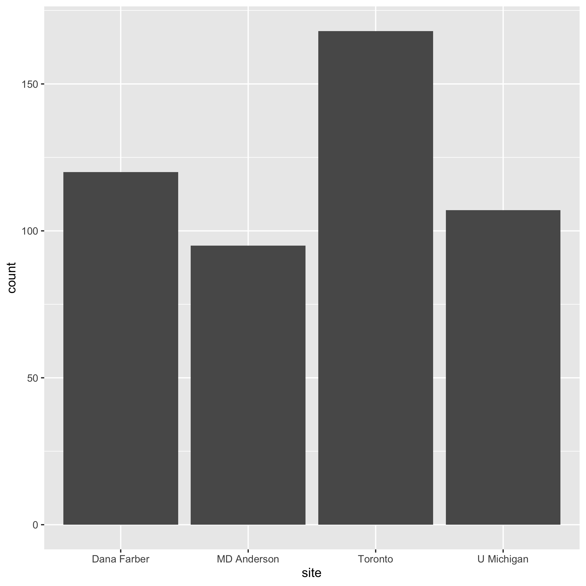
We can look at the the text output of our metadata tibble and we can use the count function to see the number of subjects that came from each center, but that quickly becomes tedious. Bar plots are a good option for visualizing these types of data. Let’s generate a bar plot of the number of subjects at each center. We’ll see that the syntax for making a bar plot is analogous to what we did in the previous lesson to make a scatter plot. To make a basic bar plot, the only aesthetic we need to provide is the variable we’d like along the x-axis:
ggplot(metadata, aes(x=site)) +
	geom_bar()
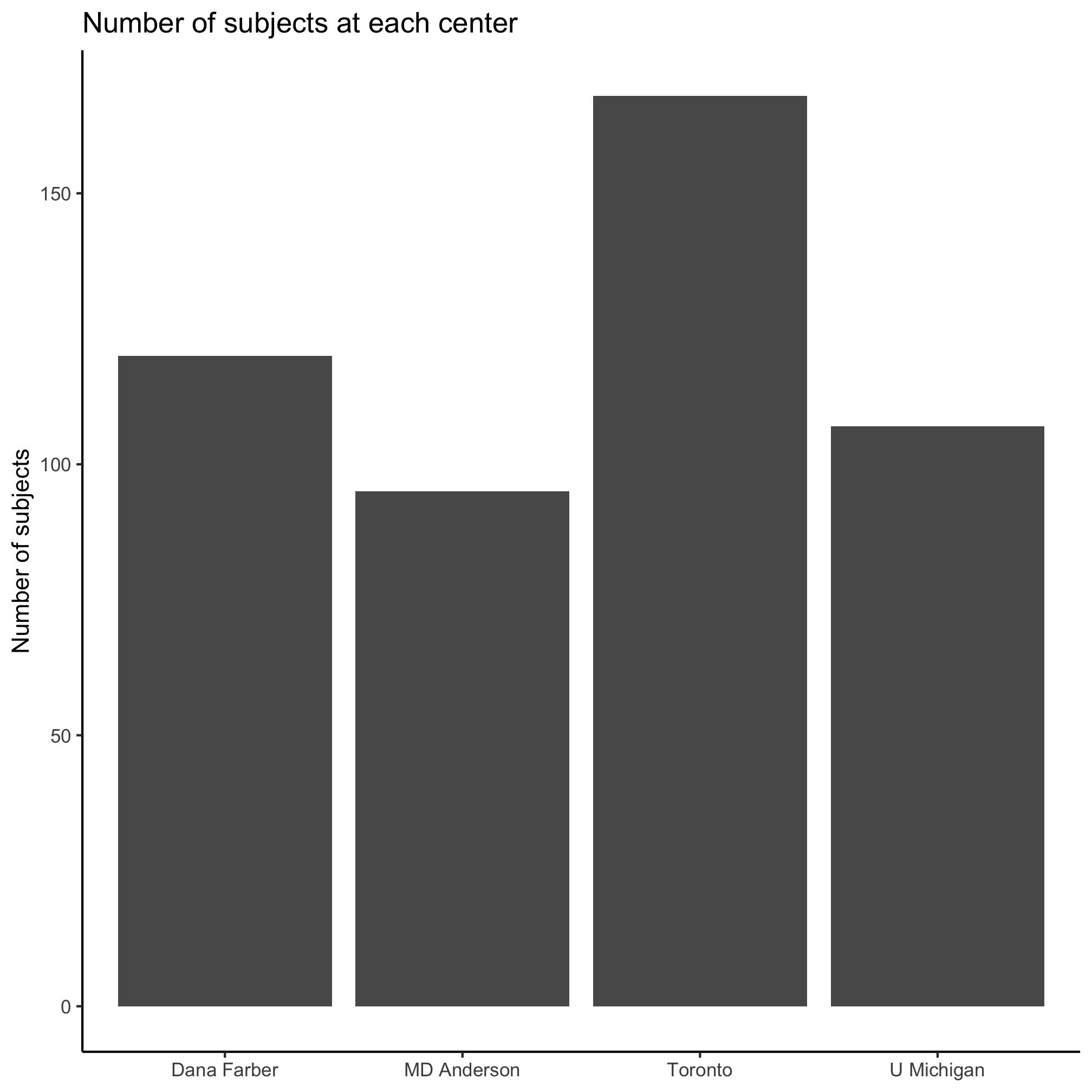
With some of the same commands we used previously, we can get this to look a little nicer
ggplot(metadata, aes(x=site)) +
	geom_bar() +
	labs(title="Number of subjects at each center",
		x=NULL,
		y="Number of subjects") +
	theme_classic()
Nice. Let’s say we want to know the number of male and female patients at each site. To do this we will use the color aesthetic to color the bars by sex. The bars will be grouped along the x-axis by site and then by sex.
ggplot(metadata, aes(x=site, color=sex)) +
	geom_bar() +
	labs(title="Number of male and female subjects at each center",
		x=NULL,
		y="Number of subjects") +
	theme_classic()
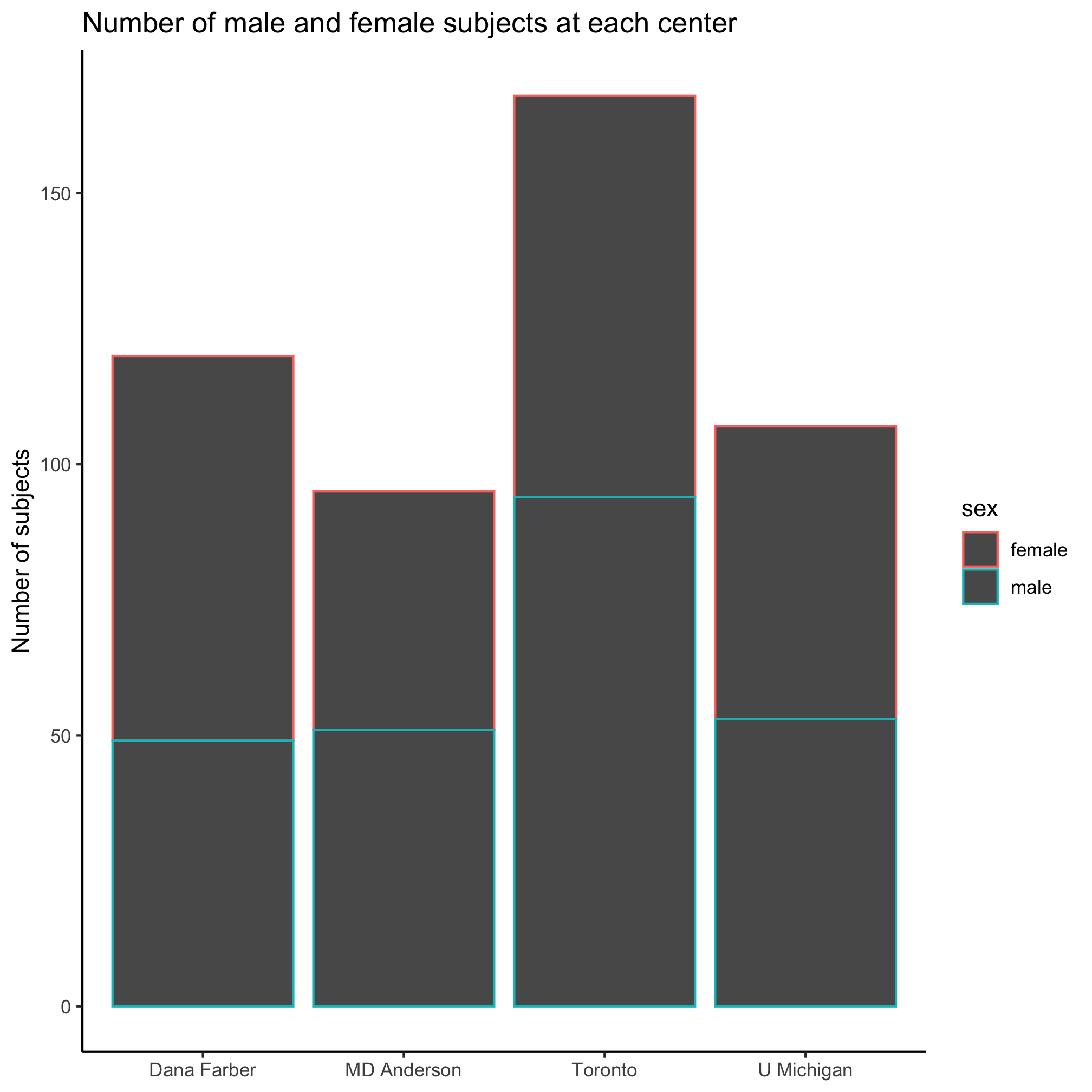
Huh. That looks weird. It appears that the border of the bars was colored rather than the content of the bar. It also appears that the male and female bar for each center were stacked on top of each other. We’re not big fans of stacked bar plots and we’d really like these bars to be side-by-side. Go ahead and run ?geom_bar and scroll down to the “Aesthetics” section of the help page. Do you see any aesthetics that might help us color the inside of the bars? If you can’t figure it out, scroll down further to find the “Examples” section and look at how they suggest using the geom_bar command. Can you figure out which aesthetic will change the interior color? Hopefully, you’ve figured out that it should be the fill aesthetic instead of the color aesthetic.
ggplot(metadata, aes(x=site, fill=sex)) +
	geom_bar() +
	labs(title="Number of male and female subjects at each center",
		x=NULL,
		y="Number of subjects") +
	theme_classic()
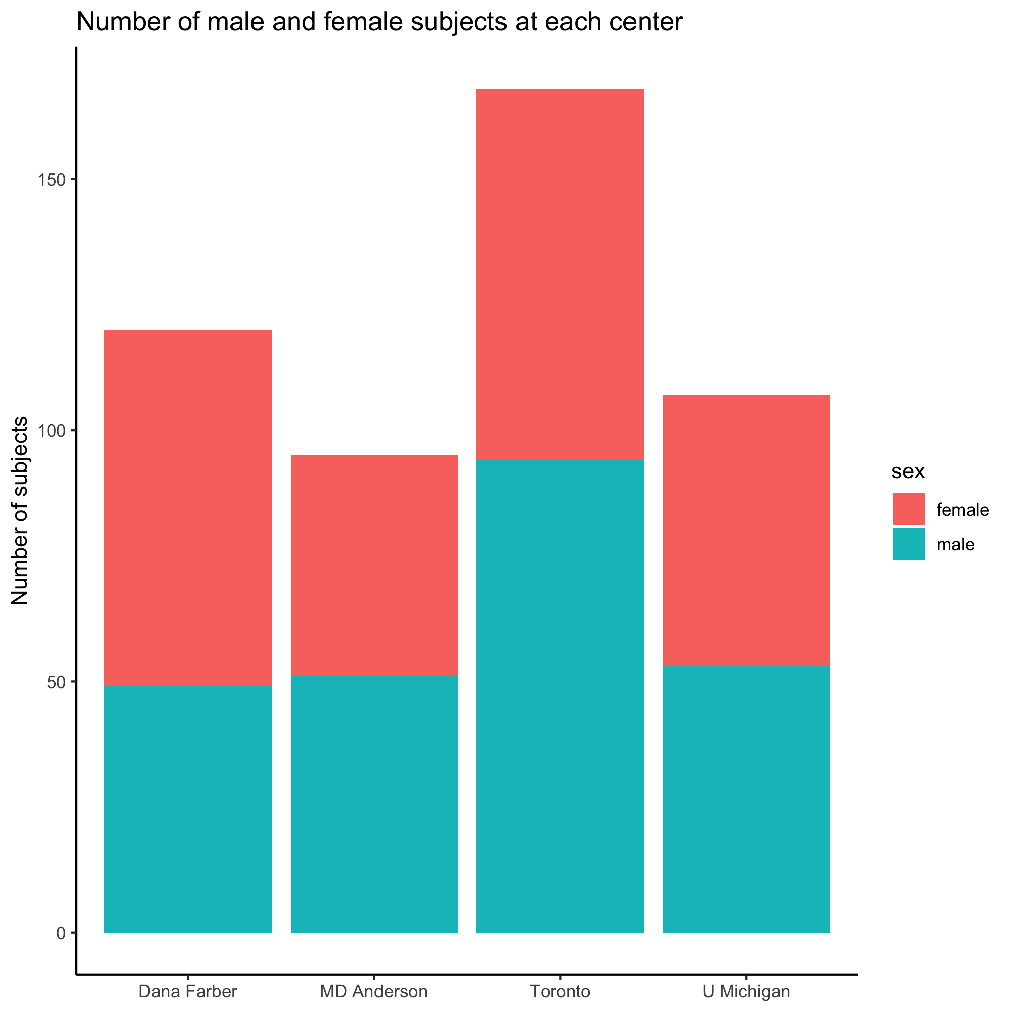
Great, we’ve solved the problem of how to set the fill color. Now we need to figure out how to stop the bars from stacking. Looking back through the ?geom_bar help page, do you see anything that tells you how to plot the bars next to each other instead of on top of each other? As a hint, look at the “See Also” section. It indicates that we should see “‘position_dodge()’ and ‘position_dodge2()’ for creating side-by-side bar charts.” OK. Now let’s do ?position_dodge to see what this is all about. In the “Examples” section, we see an example that uses position_dodge with geom_col. Nice.
ggplot(mtcars, aes(factor(cyl), fill = factor(vs))) +
 geom_bar(position = "dodge2")

# By default, dodging with `position_dodge2()` preserves the total width of
# the elements. You can choose to preserve the width of each element with:
ggplot(mtcars, aes(factor(cyl), fill = factor(vs))) +
 geom_bar(position = position_dodge2(preserve = "single"))
After playing around with position_dodge and position_dodge2 and their various options, we might settle upon this
ggplot(metadata, aes(x=site, fill=sex)) +
	geom_bar(position = position_dodge()) +
	labs(title="Number of male and female subjects at each center",
		x=NULL,
		y="Number of subjects") +
	theme_classic()
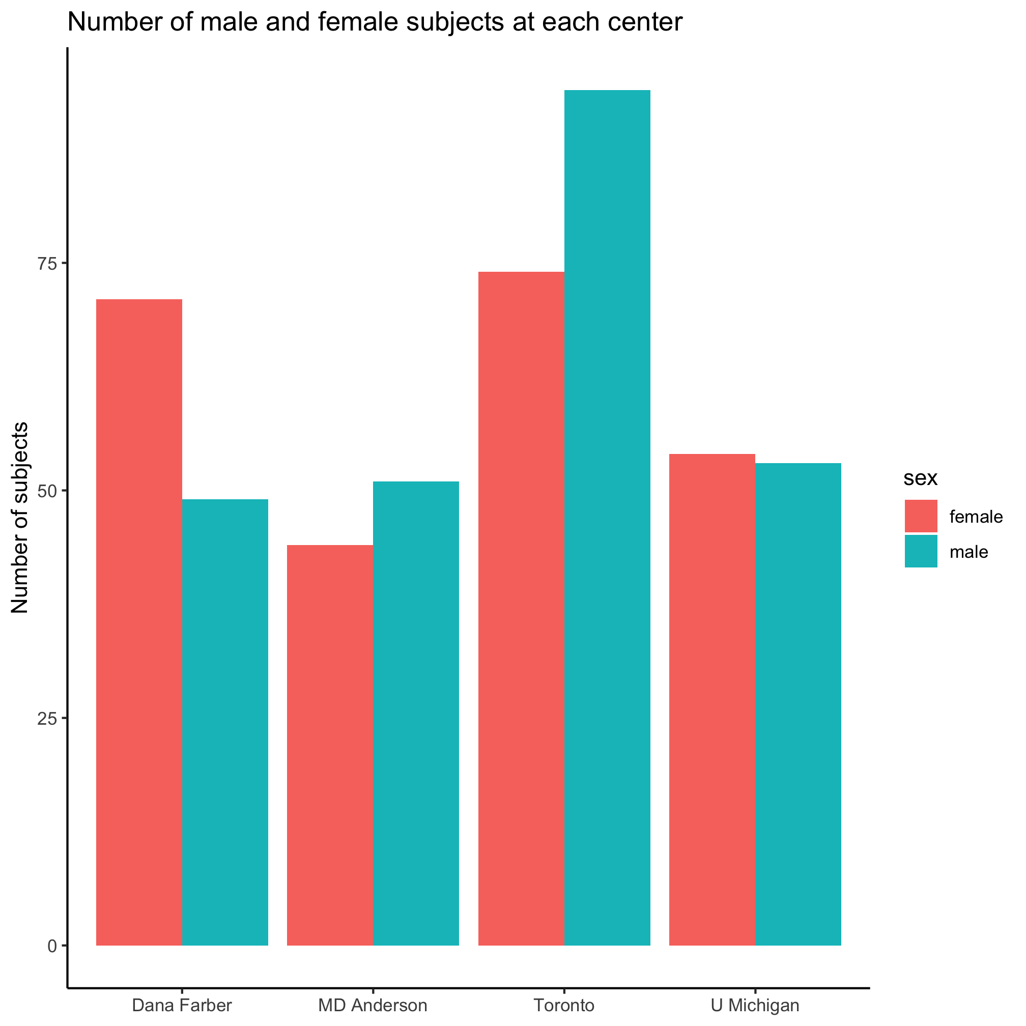
I’m not a fan of the default colors, having a legend title, or of the formatting of “female” and “male”. I’d rather use some different colors, leave out the legend title, and capitalize the first letter of the two sexes. Previously, we set the color of the diagnosis groups using scale_color_manual. We can do the same thing for our bar plot using scale_fill_manual. Can you see the difference?
ggplot(metadata, aes(x=site, fill=sex)) +
	geom_bar(position = position_dodge()) +
	scale_fill_manual(name=NULL,
		values=c("lightgreen", "purple"),
		breaks=c("female", "male"),
		labels=c("Female", "Male")) +
	labs(title="Number of male and female subjects at each center",
		x=NULL,
		y="Number of subjects") +
	theme_classic()
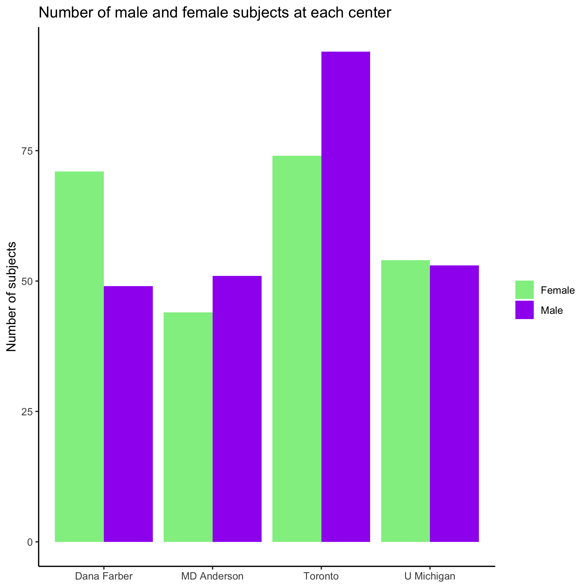
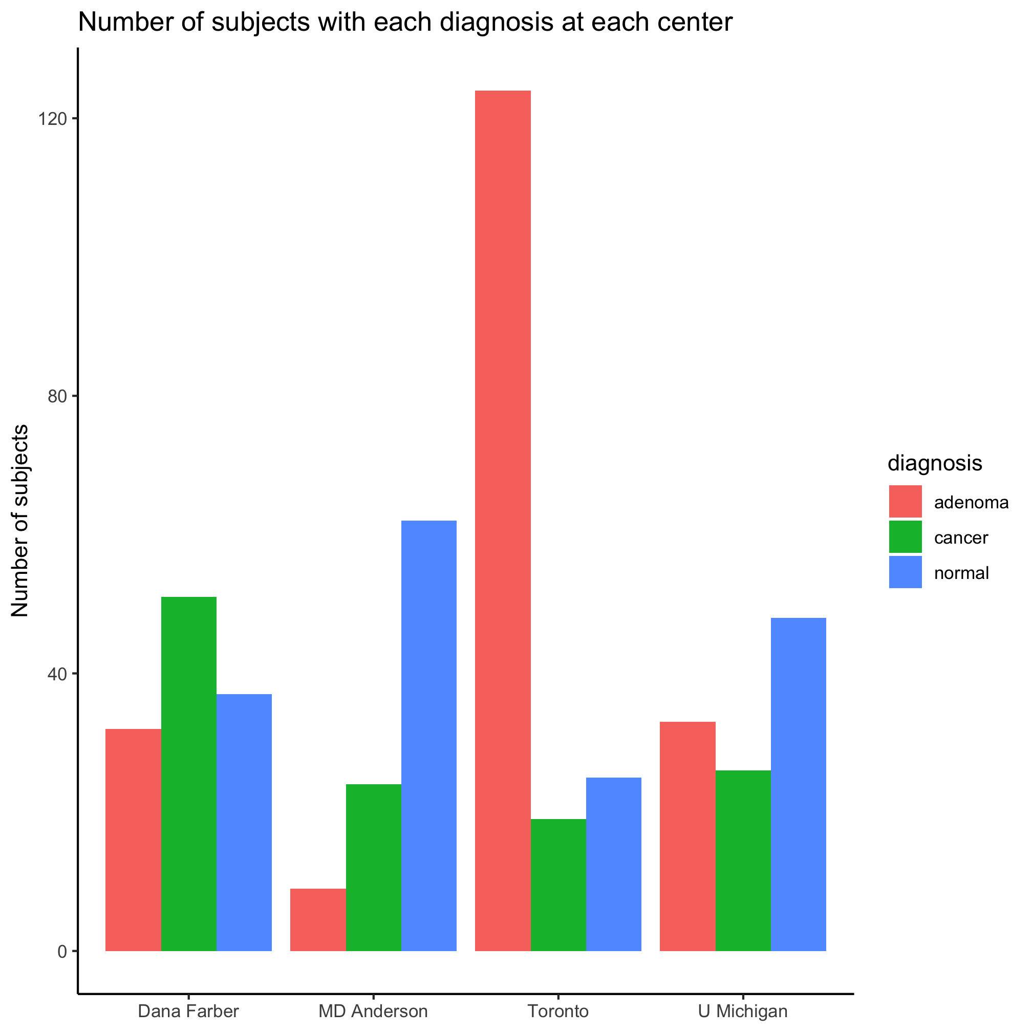
Nice, eh? Ok, so the colors aren’t amazing. Now let’s ask a different question, how are the three diagnosis groups distributed within each center? We can start simple
ggplot(metadata, aes(x=site, fill=diagnosis)) +
	geom_bar(position = position_dodge()) +
	labs(title="Number of subjects with each diagnosis at each center",
		x=NULL,
		y="Number of subjects") +
	theme_classic()
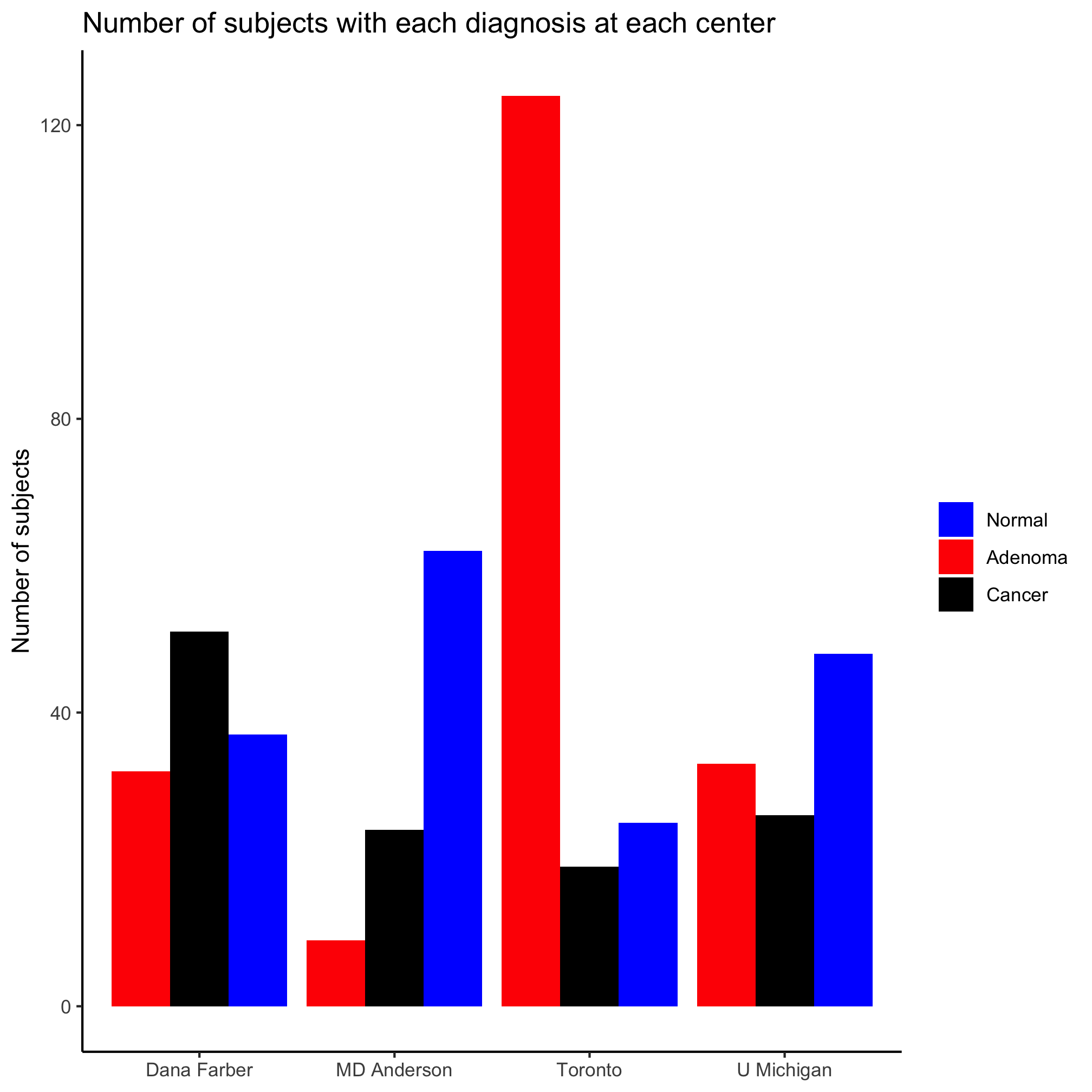
We can add our scale_fill_manual like we did earlier
ggplot(metadata, aes(x=site, fill=diagnosis)) +
	geom_bar(position = position_dodge()) +
	scale_fill_manual(name=NULL,
		values=c("blue", "red", "black"),
		breaks=c("normal", "adenoma", "cancer"),
		labels=c("Normal", "Adenoma", "Cancer")) +
	labs(title="Number of subjects with each diagnosis at each center",
		x=NULL,
		y="Number of subjects") +
	theme_classic()
Factors
You may notice that the order of the diagnosis labels is correct in the legend, but not along the x-axis. We can fix this problem by adding a line of code and reordering the colors in the line with the values argument.
metadata <- mutate(metadata, diagnosis = factor(diagnosis, levels=c("normal", "adenoma", "cancer")))

ggplot(metadata, aes(x=site, fill=diagnosis)) +
	geom_bar(position = position_dodge()) +
	scale_fill_manual(name=NULL,
		values=c("black", "blue", "red"),
		breaks=c("normal", "adenoma", "cancer"),
		labels=c("Normal", "Adenoma", "Cancer")) +
	labs(title="Number of subjects with each diagnosis at each center",
		x=NULL,
		y="Number of subjects") +
	theme_classic()
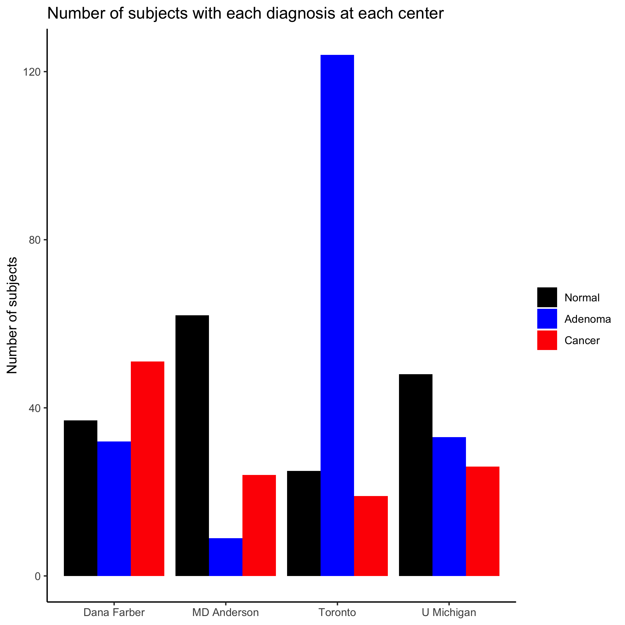
We turned diagnosis from an unordered categorical variable into an ordered categorical variable, an ordinal variable. In R these are called factors and we’ll talk about them more later. They’re one of the more frustrating parts of R for beginners and experts. You should also notice that we also put the colors in scale_fill_manual into the desired order.
Activity 9
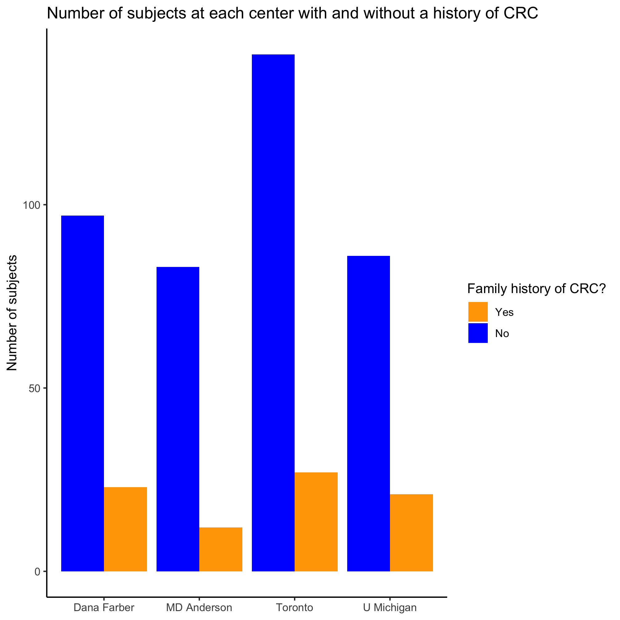
Create a bar plot that shows the number of people with and without a family history of colorectal cancer at each of the centers
Activity 10
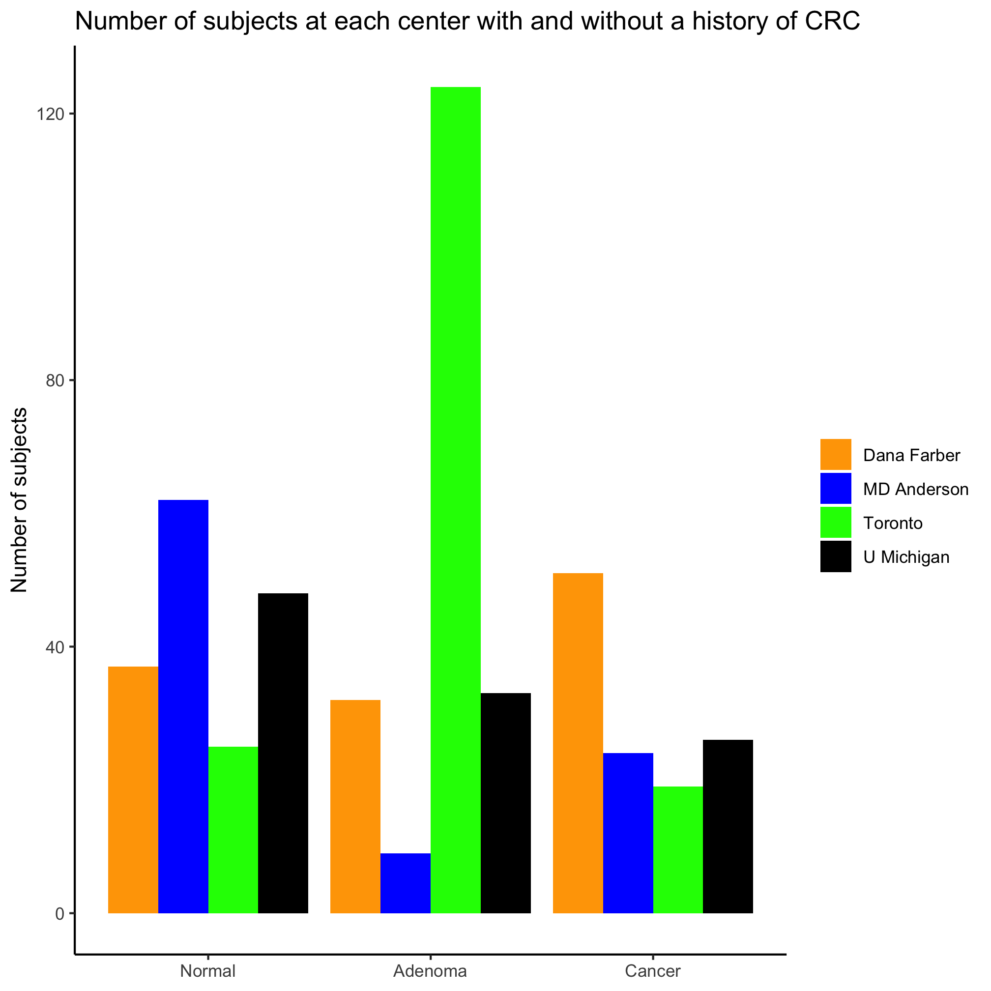
Above we plotted the site along the x-axis with diagnosis as the secondary variable. Switch it so that diagnosis is plotted along the x-axis and the site is the secondary variable. Which version of the plot do you prefer? When would you chose one orientation over the other?
